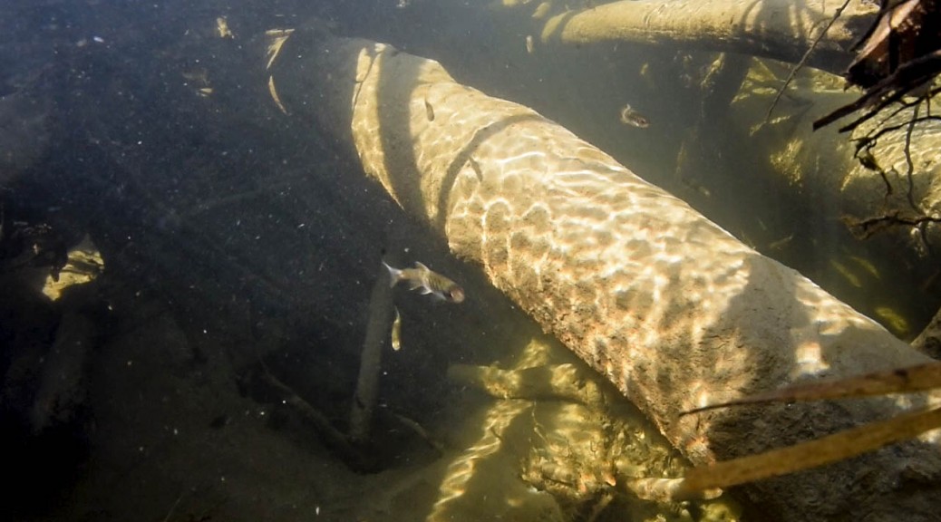
I was processing video data from this summer and thought this frame was especially pretty, so I polished it up a bit in Photoshop.
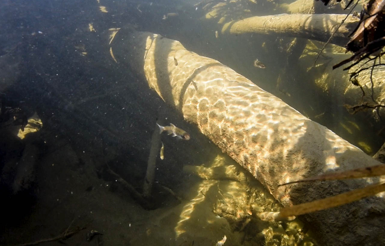
I was processing video data from this summer and thought this frame was especially pretty, so I polished it up a bit in Photoshop.
A model we’re developing examines the idea that the behavior of drift-feeding fish is largely determined by cognitive limits on their ability to process visual information. We’ve hypothesized that the fish focus their efforts on a particular region (for example, within a 10 cm radius of their snout), or on particular types of prey, to avoid sensory overload from trying to search too much space or sort through too many drifting items at once. Even with this focus, 91% of the foraging maneuvers of juvenile Chinook salmon in the Chena River are directed at items they reject (by abandoning the chase or spitting things out), and it’s obvious on video that there’s far more debris present than what the fish actually pursue.
But how much is there, exactly?
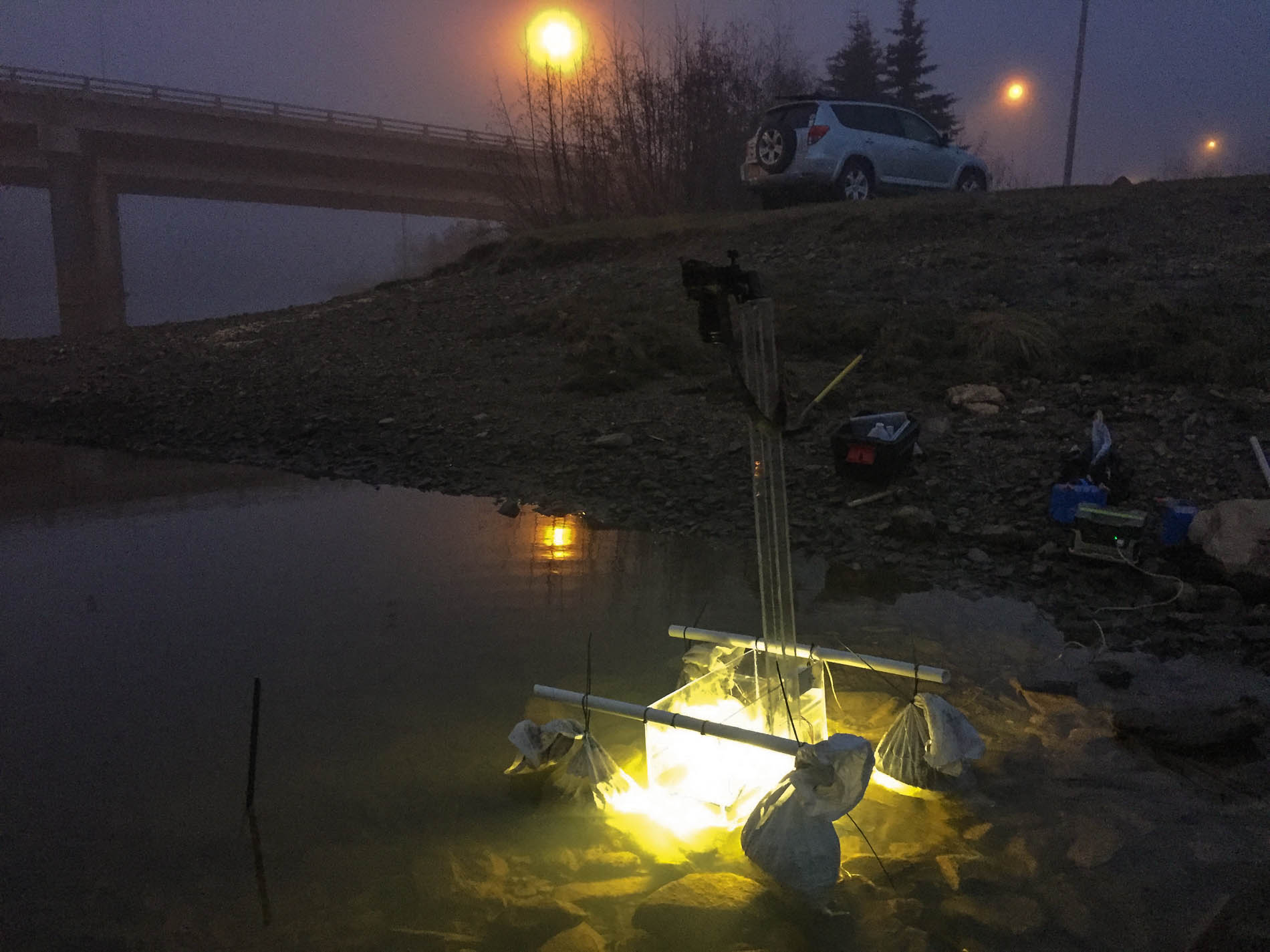
It’s easy to collect the debris with a drift net and weigh it, but that doesn’t tell us how many pieces there were, nor how big they were — both crucial pieces of information for understanding the visual challenge facing a fish as it tries to locate prey amongst the debris. To get that information, we’re developing a new technique based on computer vision. We use a DSLR to take thousands of pictures of water flowing through a well-lit rectangular chamber against a dark background. Here’s the first version of that contraption in the Chena River a few days ago:
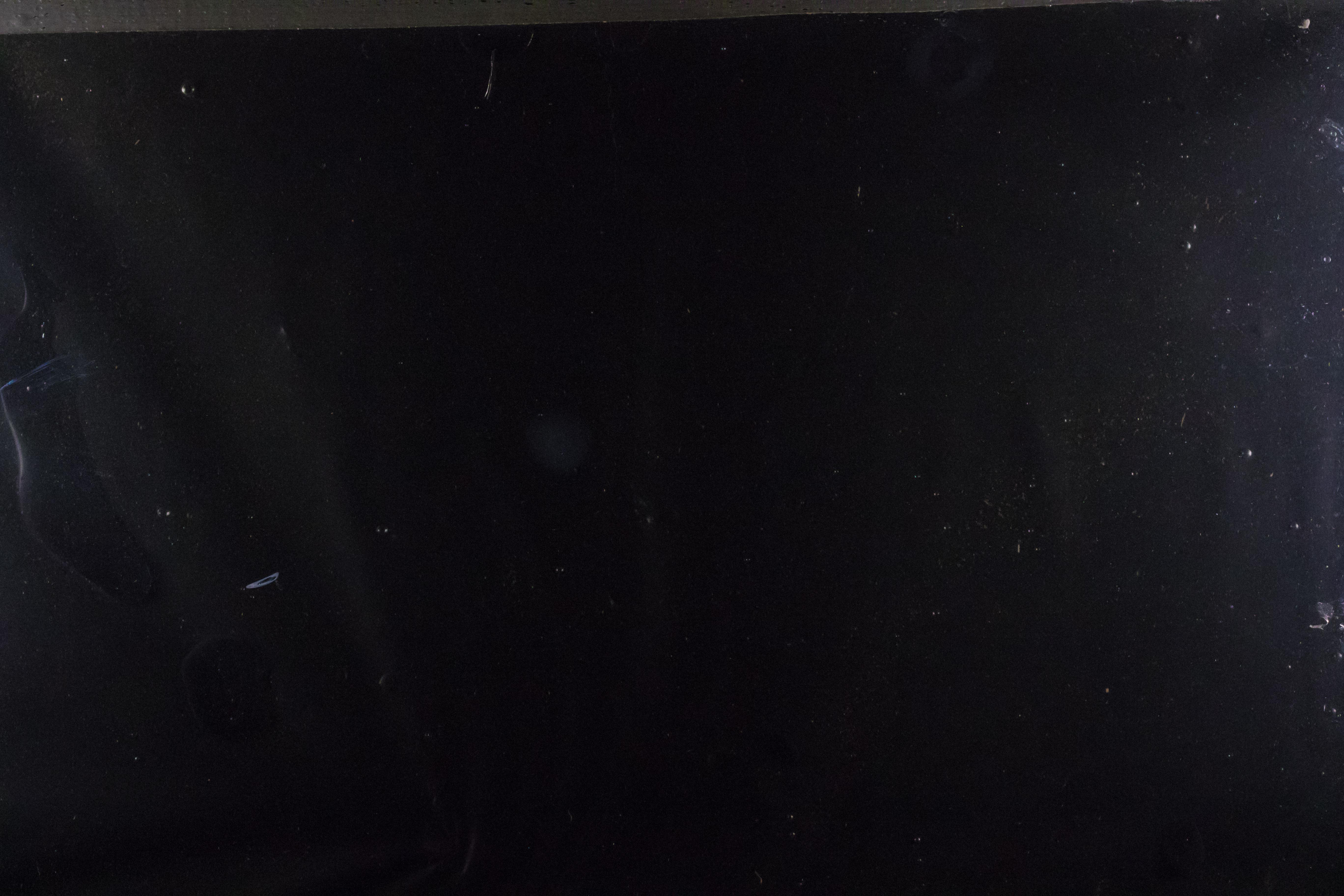
 We took a picture per second to get around 2,500 pictures that look like this (click it to view full size):
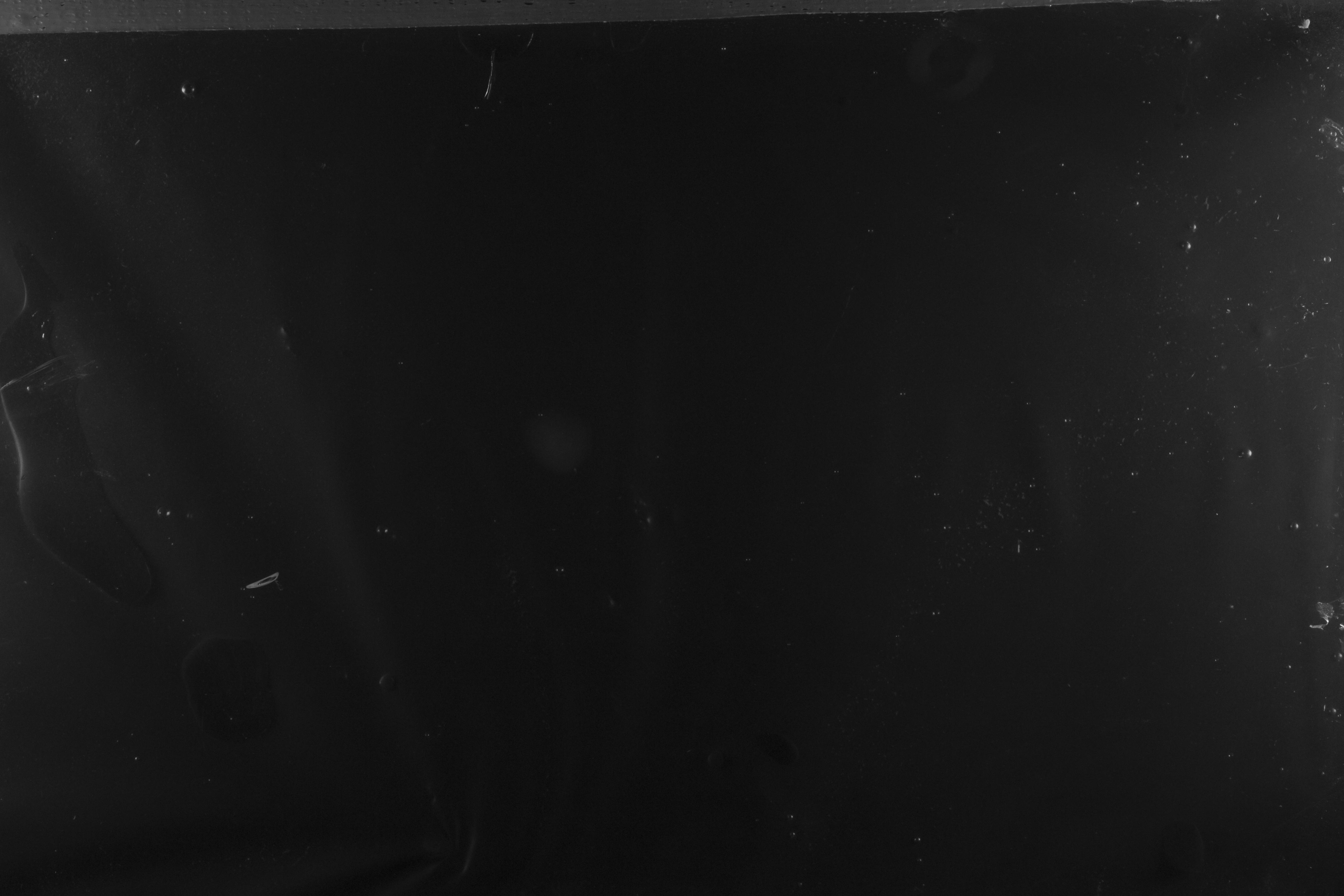
Most of that junk against the black background is stuck to the chamber somehow, not actual drifting debris. We can get a picture that excludes the real drifting stuff (or anything that’s moving) by taking the average (median) of ten consecutive pictures, a technique borrowed from astronomy. Here’s the average (which was also converted from color to grayscale to speed up the calculations):
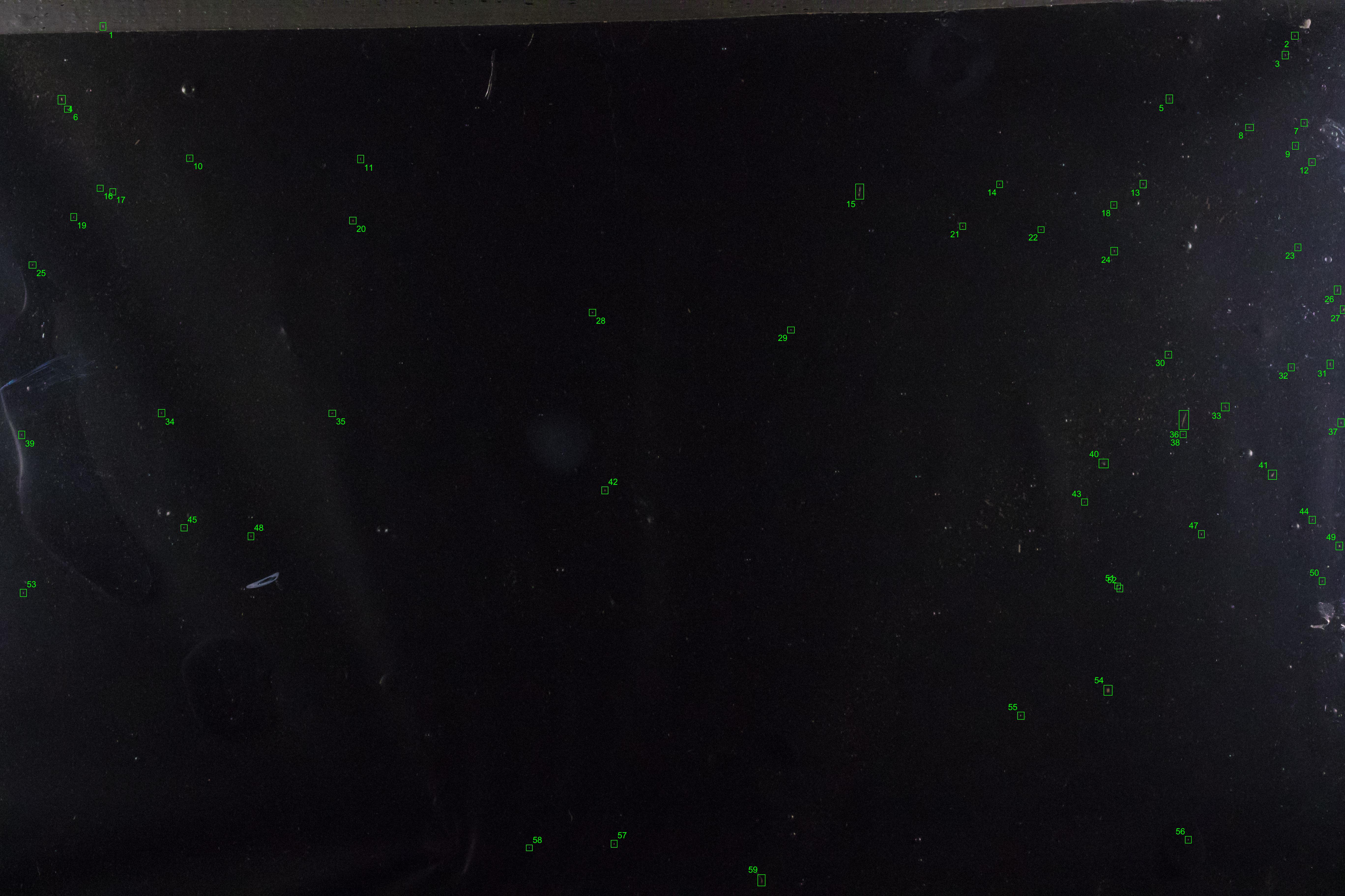
 It hardly looks any different. But if we subtract this background from one of the individual images containing drifting items, we theoretically get an image with only the drifting items. The reality is a bit messier, because some of the non-drifting items change slightly in appearance between frames and can show up in the subtracted image, but we have a nice bag of tools for dealing with that. In the end, the process lets us pick out almost all the drifting debris, highlighted and numbered in green boxes in the image below:
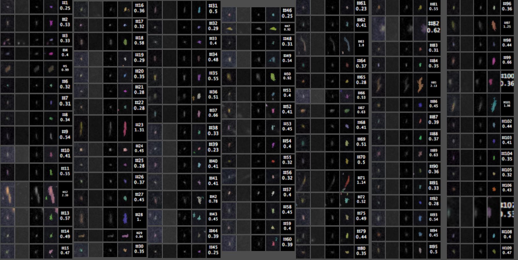
 The detected particles can then be counted and measured. Here are the close-ups, with the index # of each particle listed above its length in millimeters. The four images of each particle, from left to right, are from (1) the original image, (2) the median background, (3) the original minus the median background, and (4) a false-color overlay showing which pixels were actually counted as part of the particle.
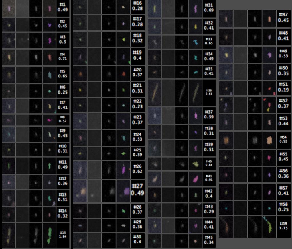
Here’s another one, just because they’re pretty:
It takes about 30 seconds for the computer to crunch one image, so an overnight program run will allow us to count and measure tens of thousands of debris particles from several cubic meters of water.
We won’t need to do this every time we go in the field to observe fish. The particle size composition and average weight per particle probably don’t change too much within each stream at normal water levels, although they may be very different in different streams. So we’re planning to run this system alongside a drift net, a few times per stream, to establish relationships between weight of debris in the net and debris counts/sizes from the images. Then we’ll be able to reasonably infer debris counts and sizes based on debris weights in the nets at all our other study sites.
This was the very first test of this whole idea, and as expected there are some little problems, like a roughly hourglass-shaped region in the middle of the image where not all the debris particles were detected. We have easy fixes for every problem identified so far, and are going to get some really interesting data when we deploy this system in the field next summer.
Our fieldwork consists of recording feeding fish on video, then capturing them (or their neighbors, if necessary) and harmlessly collecting their stomach contents to see what they ate during our observations. We’ll then compare these data with model predictions. We take photos of each fish we stomach sample, from both sides, so we can compare their appearances (spots, parr marks, scars, etc.) and see which stomach samples correspond to which fish we observed on video.
We also accomplish two tasks at once by photographing each fish against a ruler-like grid to measure its length. We started out with a storebought 1/8-inch grid (pink in the pictures), but then used custom black and white metric grids for most of the summer (with progressively thicker marks at 1, 10, and 100 mm).
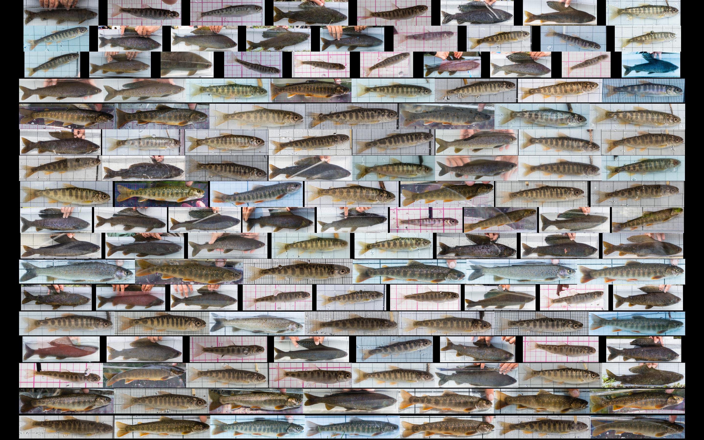
After using photo software (Lightroom) to crop/straighten all the fish images and add metadata (such as species, length, and left/right view) I sent the whole batch to Mathematica to organize all the metadata into spreadsheets and generate some graphics. Here are all the fish we physically sampled this summer, from the left (click the image to see it full-size):
 And the other side of all the same fish:
 And here are collages of each species, with image size being proportional to the size of the fish. Juvenile Chinook salmon:
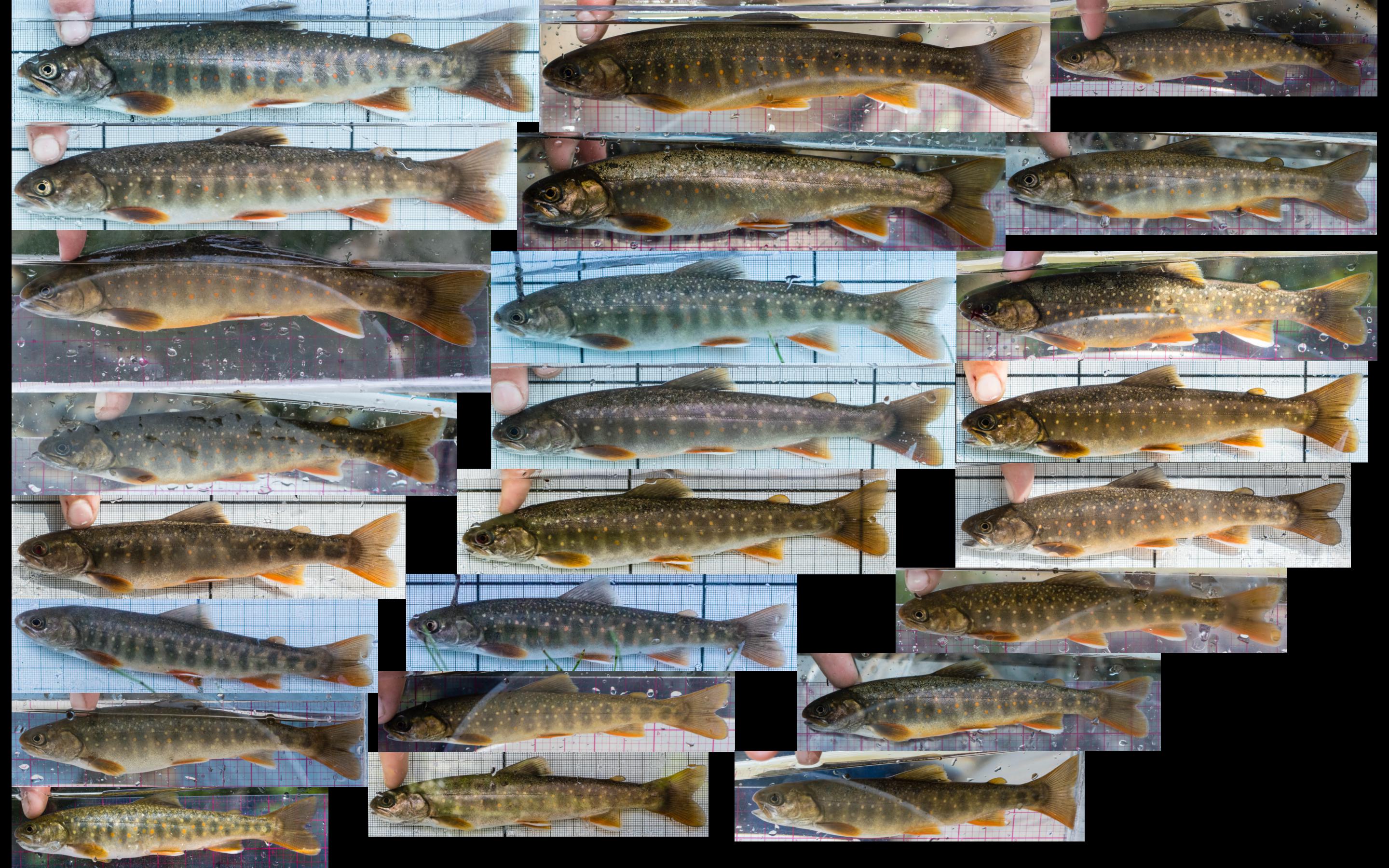
 Dolly varden:
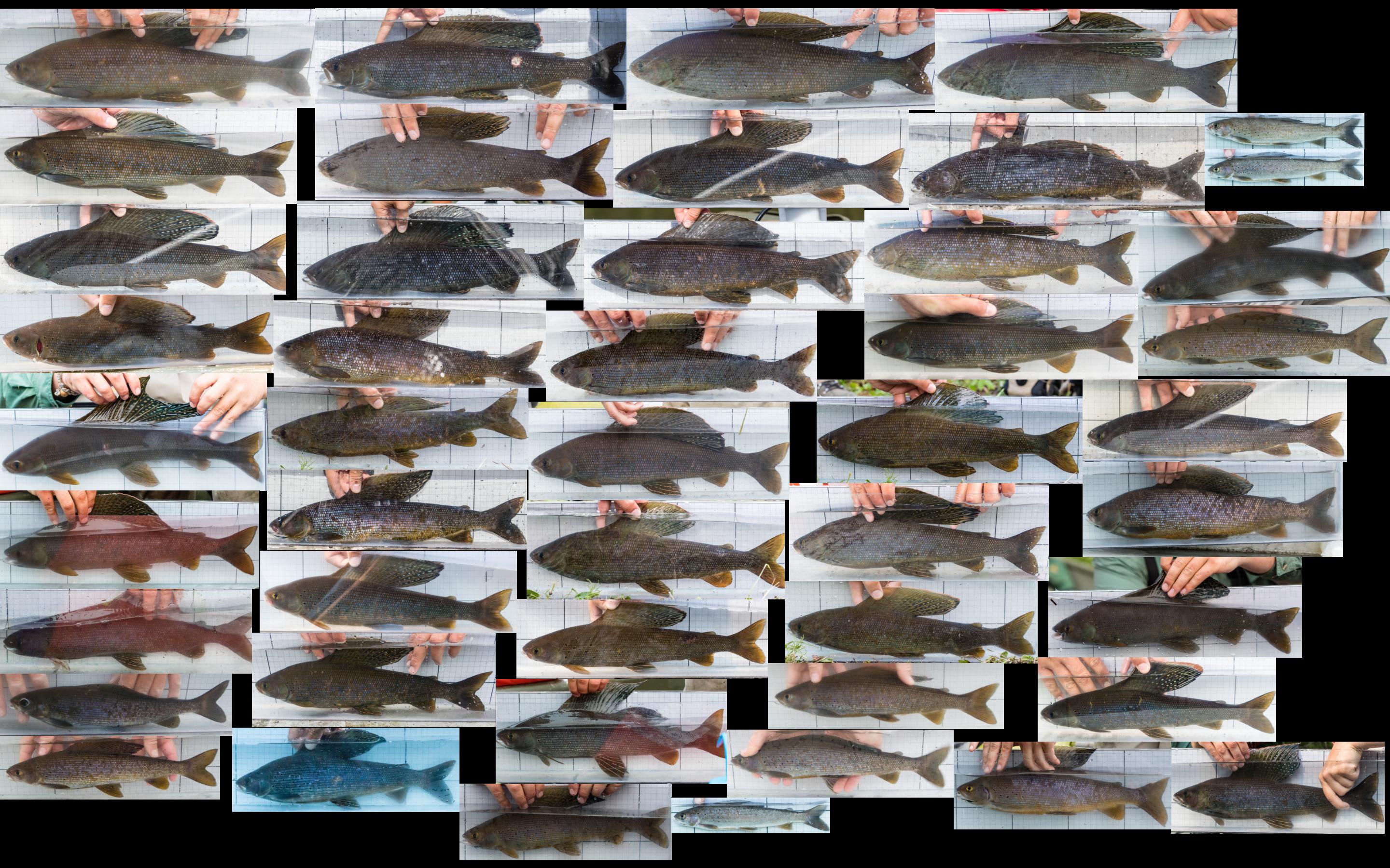
 Arctic grayling:
 The above images are mostly just for fun. The main application of these images, besides length measurement, is to group them into “reference cards” for comparing fish on video to the fish we caught at each of our 31 study sites. Here are a couple of those, showing each fish from both sides: